CDP Simulator Examples

Here are some examples of how to implement the simulation model.

• The first example is a mass-spring system, starting with one simple mass-spring. For the simple mass-spring, multiple solutions are presented: code-based, no-code and low-code. The code-based solution is then extended to `N` masses, using state variable arrays and reaching the limit of real-time performance.
• The second example deals with a rotary inverted pendulum, including a controller design. Two solutions are presented: one using ordinary differential equations (ODEs) and the other using differential-algebraic equations (DAEs).
• The third is simulating a long elastic wire, putting the integration algorithms to the test.

For instructions on how to create the simulator project, follow the Getting Started.

Example 1: Mass Hanging from a Spring

Simple Mass-spring

Mathematical model:

`dot x = v`

`dot v = g − x k/m`

Follow the instructions to get started. Add two state variables: position (`x`) and speed (`v`) using the CDP Studio, as described in the previous chapter. Then, add parameters for the spring constant (`k`), mass (`m`) and gravity (`g`). In Code mode, implement the method EvaluateDiffEquations(). It would be something like this:

void YourModelName::EvaluateDiffEquations(double t)
{
    x.ddt = v;
    v.ddt = g - x * k/m;
}

The position `x` denotes the displacement from spring equilibrium. Due to gravity, the equilibrium for the mass-spring system will be a distance `x_0 = mg/k` below this point. Since the state variables have an initial value of zero, the initial acceleration is `g`, and the system will start oscillating immediately.

To let the system start at rest, let instead `x` denote the displacement from system equilibrium. Replacing `x` by `(x + x_0)` in the expression for `v.ddt` reduces the expression to v.ddt = - k/m * x;. You now have to excite the mass to make your system run, set for example `x = 1` from CDP Studio Configure mode when connected to the system.

void YourModelName::EvaluateDiffEquations(double t)
{
    x.ddt = v;
    v.ddt = - k/m * x;
}

No-code Simple Mass-spring

To create the same simple mass-spring system without writing any code, go to Configure mode Block Diagram and follow these steps:

• In the simulator application, add a CDPSim.SimComponent from the Resource tree and name it MassSpring.
• Navigate into the MassSpring component.
• Add the following CDPParameters to the MassSpring component from the Resource tree:
  • Add CDPCore.CDPParameter k (spring constant) and set its Value property to 1.
  • Add CDPCore.CDPParameter m (mass) and set its Value property to 0.5.
• Add the following output signals to the MassSpring component:
  • Add CDPSim.SimSignal v (speed) and set its Input property to false.
  • Add CDPSim.SimSignal x (displacement) and set its Input property to false.
• Add two integrators to the MassSpring component which will integrate the displacement to get the speed:
  • Add CDPSim.Integrator Velocity.
  • Add CDPSim.Integrator Displacement.
• Add the following CDPOperators to the MassSpring component:
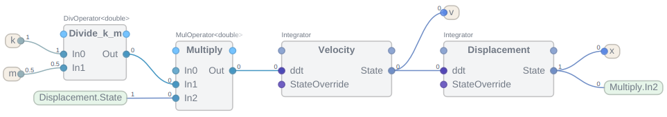
  • Add Automation.Divide<double> and name it Divide_k_m. Connect the two inputs to the k and m parameters.
  • Add Automation.Multiply<double>. Next, add a third CDPCore.Argument<double> named In2. Finally, set In0 to -1, connect the Divide_k_m output to In1, and connect the Displacement.State output to In2.
• Add the missing connections:
  • Connect the Multiply output to the Velocity.ddt input.
  • Connect the Velocity.State output to the Displacement.ddt input.
  • Connect the Displacement.State output to the x SimSignal.
  • Connect the Velocity.State output to the v SimSignal.

The final configuration will look like this:

Low-code Simple Mass-spring

For the low-code solution, we will take the no-code solution and do the following changes:

• Remove the Divide_k_m and Multiply operators.
• Add the Automation.Evaluate<double> operator.
• Add 3 CDPCore.Argument<double> named k, m and x to the Evaluate operator.
• Set the Expression property of the Evaluate operator to:

  -k/m * x

• Add the missing connections:
  • Connect the Evaluate.Out to the Velocity.ddt input.
  • Connect the Displacement.State output to the x SimSignal.
  • Connect the Velocity.State output to the v SimSignal.

The final configuration will look like this:

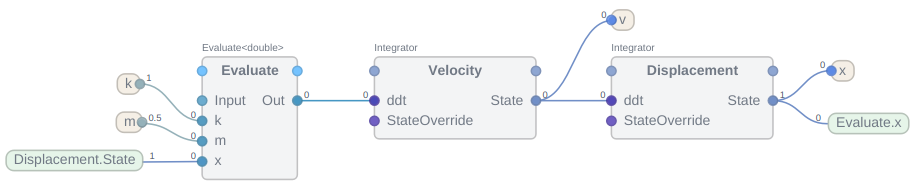
The main benefit of the low-code solution is that you can easily change the expression in the Evaluate operator and implement a more complicated model without adding too many operator blocks - for example when adding damping, one would need many more blocks in the no-code solution.

Limiting Spring Movement

Consider that space is limited, for example, the mass is hanging above a table and will hit it if displacement becomes too large. First, add a parameter for the position of the table (x_table) and set it to a suitable value, for example, x_table = 0.5.

For the C++ code-based solution, check the position of the mass in the PostIntegrate() method:

void YourModelName::PostIntegrate()
{
    if (x < x_table)
    {
        x.OverrideStateValue(x_table);
        v.OverrideStateValue(0); // Reset speed to 0 after hitting the table
    }
}

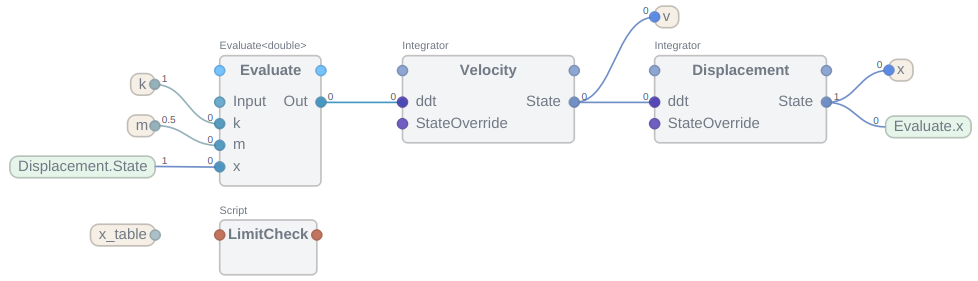
For the no-code and low-code solutions made in the previous step, the post-integration condition can be set using the Script block.

Navigate into the MassSpring SimComponent and add a CDPSim.Script LimitCheck. Click on the script block and edit the following properties:

• Set Execution to 3 - PostIntegrate. This will make the script run right after the integration step.
• Set Script to the following ChaiScript code:

  if (Displacement.State < x_table) {
      Displacement.State = x_table;
      Velocity.State = 0; // Reset speed to 0 after hitting the table
  }

The final configuration will look like this:

Damping

This oscillating system will go on forever. In reality, there will always be some drag forces causing a damping of the oscillations. In this mass-spring system, a viscous damping force `F = -bv` due to air drag and spring friction will be present. To include damping in your model, add a parameter `b` (damping coefficient) from Code mode, and rewrite EvaluateDiffEquations() like this:

void YourModelName::EvaluateDiffEquations(double t)
{
    x.ddt = v;
    v.ddt = -x * k/m - v * b/m;
}

To check the validity of the simulation generated by CDPSim, read out the undamped oscillatory period (time between extrema) from the graph, and compare with the theoretically calculated period.

`T = 2 pi sqrt{m/k}`

Two Masses and Two Springs Coupled in Series

Follow the instructions to get started. In this case, you need four state variables: positions (`x1` and `x2`) and speeds (`v1` and `v2`). Add these in the Code mode. For simplicity, assume that both the two masses and the two springs are equal. Add parameters for the spring constant (`k`) and mass (`m`) in the Code mode. A suitable choice of parameter values might be `k = m = 1`. Let `x1` and `x2` denote the displacements from the equilibrium points for the masses, such that this oscillating system becomes independent of the gravity (The gravity would only influence the location of the equilibrium points, and not the displacements, due to linearity in Hookes law). In Code mode, implement EvaluateDiffEquations() like this:

void YourModelName::EvaluateDiffEquations(double t)
{
    x1.ddt = v1;
    x2.ddt = v2;
    v1.ddt = k/m * (x2 - 2*x1);
    v2.ddt = k/m * (x1 - x2);
}

As in the previous example, damping can be included simply by adding a parameter `b` (damping coefficient) and adding a term `-b/m*v` in the expression for `v1.ddt` and `v2.ddt`:

v1.ddt = k/m * (x2 - 2*x1) - b/m * v1;
v2.ddt = k/m * (x1 - x2) - b/m * v2;

N Masses and Springs Coupled in Series (Using Arrays)

Follow the instructions to get started. It is suitable to use state variable arrays for the positions and speeds. First, add the parameters `k` and `m`. In addition, add a parameter `n` (larger than 1) to denote the number of masses in the system. Then manually implement the rest of the code.

Under the parameter declarations, declare the state variable arrays like this:

CDPSim::StateVariableArray x;
CDPSim::StateVariableArray v;

Open YourLibName->Sources->YourModelName.cpp. First, in the Configure() method, make sure that the size of arrays n is set at startup. Then create the x and v arrays like this (the last argument denotes the size of the arrays):

void YourModelName::Configure(const char* componentXML)
{
    DynamicSimComponent::Configure(componentXML); // Initializes `n`
    if (n < 2)
        n = 2;
    n.AddNodeModeFlags(CDP::StudioAPI::eValueIsReadOnly); // `n` can't be changed at run-time
    x.Create("x", this, n);
    v.Create("v", this, n);
}

In EvaluateDiffEquations(), implement the differential equations for the system. It can be done this way:

void YourModelName::EvaluateDiffEquations(double t)
{
    x[0].ddt = v[0];
    x[x.Size()-1].ddt = v[v.Size()-1];
    v[0].ddt = k/m * ( x[1] - 2*x[0] );
    v[v.Size()-1].ddt = k/m * ( x[x.Size()-2] - x[x.Size()-1] );
    for (int i = 1; i < x.Size() - 1; ++i)
    {
        x[i].ddt = v[i];
        v[i].ddt = k/m * ( x[i-1] - 2*x[i] + x[i+1] );
    }
}

Now run your model. You have to excite the mass to make your system run, set for example `x[0] = 1` from CDP Studio Configure mode when connected to the system.

Be aware that `n` (number of masses) cannot be changed while running.

For large `n`, the real-time performance can be lost. This can be investigated by checking the NotRealTime alarm of SimulatorManager. To compensate for a large system, a larger time step for the integration can be chosen. This will be a trade-off between the real-time performance and the accuracy of the simulation.

One interesting example is to consider the system with k = 100 000 kg/s^2, m = 0.1 kg, n = 500, analogue to a wave propagating on a hanging cable. Give the first mass an initial excitation x[0] = 10. The system will have two characteristic frequencies. Now choosing time step 1e-02 results in instability of the simulation, while 1e-03 can run the system, though without real-time performance (depending on the hardware the simulator is being run on).

Example 2: Rotary Inverted Pendulum

Consider a rod mounted on a horizontally rotating arm, such that the rod rotates freely in the normal plane of the arm. The arm motion is controlled by an external torque, in order to keep the rod in an upright position. See the appendix for derivation of the differential equations.

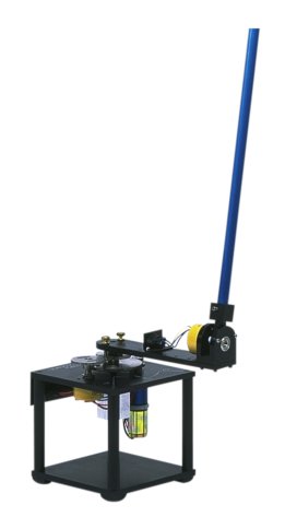
Rotary Inverted Pendulum (image courtesy, Quanser Inc. / © CC BY-SA 3.0)

Follow the general instructions to get started. From Code mode, add the following state variables: theta (angle of the rod), dtheta (angular velocity of the rod), phi (angle of the arm) and dphi (angular velocity of the arm).

Add an input SimSignal tau (external torque acting on the arm).

Now add parameters: l (rod length), r (arm length), g (gravity acceleration), m_rod (rod mass), m_arm (arm mass), c_rod (rod damping coefficient) and c_arm (arm damping coefficient).

This example will be implemented in two ways: first as an ODE system, and then as a DAE system. It is not necessary to implement both, but it is interesting to compare the two solutions. The derivation of is equations is described in the appendix.

ODE Solution

In YourLibName->Sources->YourModelName.cpp, in the EvaluateDiffEquations() method, implement the equations:

void YourModelName::EvaluateDiffEquations(double t)
{
    theta.ddt = dtheta;
    phi.ddt = dphi;

    double sin_theta = sin(theta);
    double cos_theta = cos(theta);

    // Coefficient matrix elements
    double a11 = 1.0;
    double a12 = (6.0 * r * cos_theta) / (7.0 * l);
    double a21 = 0.5 * m_rod * r * l * cos_theta;
    double a22 = r * r * (m_rod + (1.0 / 3.0) * m_arm);

    // Right-hand side terms
    double b1 = (6.0 * g * sin_theta) / (7.0 * l) - (12.0 * c_rod * dtheta) / (7.0 * l * m_rod);
    double b2 = 0.5 * m_rod * r * l * dtheta * dtheta * sin_theta + tau - c_arm * dphi;

    // Compute determinant
    double det = a11 * a22 - a12 * a21;

    if (fabs(det) < 1e-8)
    {
        // Singular matrix, set derivatives to zero
        dtheta.ddt = 0.0;
        dphi.ddt = 0.0;
    }
    else
    {
        // Solve for accelerations
        dtheta.ddt = (b1 * a22 - a12 * b2) / det;
        dphi.ddt = (a11 * b2 - b1 * a21) / det;
    }
}

DAE Solution

As an alternative to ODE, the system can be implemented as a DAE system.

In YourLibName->Sources->YourModelName.cpp, in the EvaluateAlgebraicEquations() method, implement the equations:

void YourModelName::EvaluateAlgebraicEquations(double t)
{
    theta.residual = theta.ddt - dtheta;
    phi.residual = phi.ddt - dphi;
    dtheta.residual = dtheta.ddt - (6.0 / (7.0 * l)
        * (g * sin(theta) - r * dphi.ddt * cos(theta) - (2.0 * c_rod / m_rod) * dtheta));
    dphi.residual = dphi.ddt - (1.0 / (r * r * (m_rod + (1.0 / 3.0) * m_arm))
        * (0.5 * m_rod * r * l * dtheta * dtheta * sin(theta)
            - 0.5 * m_rod * r * l * dtheta.ddt * cos(theta) - c_arm * dphi + tau));
}

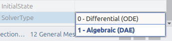
Next in Configure mode, set the SolverType property of your model to Algebraic (DAE).

Testing

You can now run your model. Choose suitable parameter values, and set for example some theta-values to check that the performance make sense.

Controller Design

The challenge is now to control the system, i.e. to keep the rod in upright position while moving the arm to a desired angle. To create a controller, add a new CDP component model to your library (not a simulator model).

When the rod is in upright position, the arm velocity is constant. To control the arm motion, the idea is to set the desired rod angle (theta) slightly different from zero, such that the arm needs to accelerate to keep the rod in this position. Many different controllers may be used, but we are in this example going to implement a simple PD-controller in order to control both the rod angle and arm angle.

Add the following input signals: theta (rod angle) and phi (arm angle). Add the output signals tau (external torque) and theta_desired (desired rod angle).

Add parameters: kg_theta (theta controller gain), kp_theta (proportional gain), kd_theta (derivative gain), kg_phi (phi controller gain), kp_phi (proportional gain), kd_phi (derivative gain), tau_max (maximum torque limit), theta_max (maximum desired angle for the rod) and phi_desired (desired arm angle).

To be able to do a swing-up maneuver if the rod falls down, add a state called Work. The code is to be implemented later. Add state transitions Null->Work (start swing-up maneuver) and Work->Null (start balancing). To manually control the swing-up, add an additional parameter called swingup_gain.

It might be useful to be able to reset the controller while running. Add a message called "Reset" with the code

tau = 0;
e_theta_prev = 0;
e_phi_prev = 0;
der_theta = 0;
der_phi = 0;
return 1;

In addition, we need some variables for computations in the code. In Code mode, open YourModelName.h, and declare the following double variables straight above the CDPParameter declarations: e_theta, e_theta_prev, der_theta, e_phi, e_phi_prev, der_phi. For example: double e_theta;

Now, open YourModelName.cpp to implement the rest of the code. In the constructor, set initial values:

YourModelName::YourModelName()
{
    e_theta = 0.0;
    e_theta_prev = 0.0;
    der_theta = 0.0;
    e_phi = 0.0;
    e_phi_prev = 0.0;
    der_phi = 0.0;
}

In the ProcessNull() method, implement this code:

void YourModelName::ProcessNull()
{
    e_theta = 0.1 * (theta - theta_desired) + 0.9 * e_theta_prev;
    der_theta = (e_theta - e_theta_prev) / ts;
    tau = kg_theta * (kp_theta * e_theta + kd_theta * der_theta);
    e_theta_prev = e_theta;
    if (tau > tau_max)
        tau = tau_max;
    if (tau < -tau_max)
        tau = -tau_max;

    e_phi = 0.1 * (phi - phi_desired) + 0.9 * e_phi_prev;
    der_phi = (e_phi - e_phi_prev) / ts;
    e_phi_prev = e_phi;
    theta_desired = -kg_phi * (kp_phi * e_phi + kd_phi * der_phi) * 0.001;
    if (theta_desired > theta_max)
        theta_desired = theta_max;
    if (theta_desired < -theta_max)
        theta_desired = -theta_max;

    if (cos(theta) < 0)
        requestedState = "Work";
}

In the ProcessWork() method:

void YourModelName::ProcessWork()
{
    e_theta = (theta - theta_desired);

    if (cos(theta) < 0)
    {
        if (e_theta > e_theta_prev)
            tau = swingup_gain*tau_max;
        if (e_theta < e_theta_prev)
            tau = -swingup_gain*tau_max;
    }
    else
        tau = 0;

    e_theta_prev = e_theta;

    if (cos(theta) > 0.8)
    {
        MessageReset(nullptr);
        requestedState="Null";
    }
}

Now the code is completed. Run the system with the simulation and controller components in Configure mode. Let the controller route theta and phi signals from the simulator, and let the simulator route the tau signal from the controller.

Tuning the controller parameters is a chapter on its own, depending sensitively on the pendulum parameters. An example of suitable values is given below.

To make the model more realistic, add a delay on the measurements of theta and phi. Go back to your simulation model in Code mode. Add a parameter called delay, and two signals called theta_output and phi_output. Then, above the parameter declarations in YourModelName.h (for the simulator, not the controller), declare these variables and functions:

public:
    virtual void PreIntegrate();
protected:
    int index; int elements;
    std::vector<double> thetas;
    std::vector<double> phis;
    double delay_old; double theta_delayed; double phi_delayed;
    virtual void ProcessNull();
    virtual void Reset();

In the constructor in YourModelName.cpp, define the variables:

{
    theta_delayed = 0;
    phi_delayed = 0;
    index = 0;
    elements = 1 + int(GetFrequency() * delay - 0.5);
    delay_old = delay;
}

Then, below EvaluateDiffEquations(), attach

void YourModelName::ProcessNull()
{
    elements = 1 + int(GetFrequency() * delay - 0.5);
    if (elements > thetas.size())
    {
        thetas.resize(elements);
        phis.resize(elements);
    }

    thetas[index] = theta;
    phis[index] = phi;
    theta_delayed = thetas[(index+1)%elements];
    phi_delayed = phis[(index+1)%elements];
    index = index + 1;
    if (index == elements)
        index = 0;
    if (delay!=delay_old)
    {
        index = 0;
        delay_old = delay;
        for(int i = 0; i < elements; ++i)
        {
            thetas[i] = theta;
            phis[i] = phi;
        }
    }
}

void YourModelName::PreIntegrate()
{
    dphi.OverrideStateValue(dphi * (1.0 - 150.0 * c_arm * GetSimulatorTimestep())); // Additional damping on the arm
    theta_output = theta_delayed;
    phi_output = phi_delayed;
}

void YourModelName::Reset()
{
    for (int i = 0; i < thetas.size(); ++i)
    {
        thetas[i] = 0.0;
        phis[i] = 0.0;
    }
    DynamicSimComponent::Reset();
}

Run the model again. Remember to change the routing from theta to theta_output, and phi to phi_output.

A set of reasonable parameters that give the desired performance is:

• l = 0.5 m
• r = 0.2 m
• g = 9.8 m/s²
• m_rod = 1.0 kg
• m_arm = 0.5 kg
• C_rod = 0.02 kg * m²/s
• C_arm = 0.02 kg * m²/s
• delay = 0.02 s
• kg_theta = 20
• kp_theta = 1
• kd_theta = 0.1
• kg_phi = 10
• kp_phi = 0.1
• kd_phi = 1
• tau_max = 5 kg * m²/s²
• swingup_gain = 0.1
• theta_max = 0.1

Also set the fs property of both controller component and SimulatorManager to 1000 Hz. The process frequency determines how fast the controller component will respond to changes in rod position.

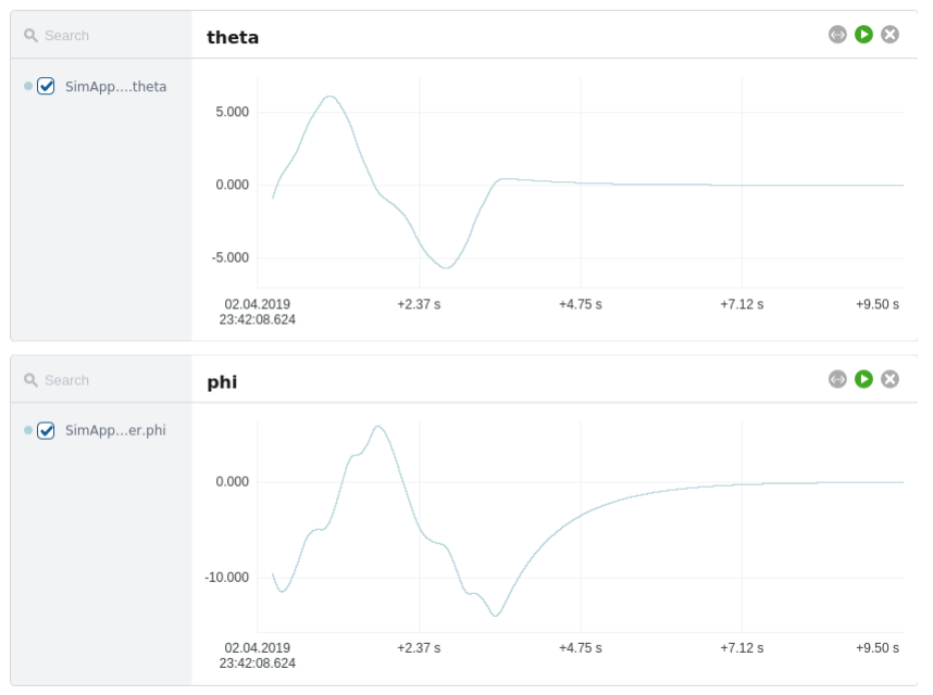
It is informative to plot theta (and sometimes tau) in one diagram, and phi in another diagram. Now set values for phi_desired and verify that the model runs as expected. Note that large delays and short rods are hard to control, but can be compensated by choosing a higher process frequency (controlled by fs property) for both controller component and SimulatorManager.

To manually adjust the controller for other pendulum parameters, start by changing kg_theta, and then kg_phi. The swing-up function should be modified in order to make it more accurate and polite.

Once the control system is capable of balancing the rod, the simulator can be used to see how changing different parameters affect its capability. Possible things to try are:

• Adjust rod length (l).
• Simulate a smaller sampling frequency of sensors. This can be done by reducing the fs property of SimulatorManager. Then signals routed between simulator and controller component are synced less frequently.
• Increase the delay parameter of simulator component. This will delay the measurements received from the simulator.
• Change initial conditions of the simulation by modifying the state variables theta and phi in the simulator component. For example setting theta to 3.14 rad means that the rod starts in "down" position.
• While simulation is running, change the phi_desired parameter of the controller component. Then the arm should take desired position after the rod has been successfully balanced.

Example 3: Long Elastic Wire

Consider a long elastic wire hanging between two masts. The wire is to be modelled by a series of `n` masses connected by `n + 1` springs. See appendix for details.

In Code mode, add parameters k (stiffness of the wire), m (mass of the wire), d (horizontal distance between masts), L (wire length at rest), g (gravity acceleration), n (number of parts the wire is divided into), h (height difference between masts) and C (damping coefficient).

Add signals wireLength (actual wire length) and mastForce (force acting on the mast from the wire) to easily read out these values while the simulation is running.

In the header file YourModelName.h, add four state variable arrays (y and v for position and speed in y direction, and x and u for position and speed in x direction):

CDPSim::StateVariableArray y;
CDPSim::StateVariableArray x;
CDPSim::StateVariableArray u;
CDPSim::StateVariableArray v;

Then add some variables for calculations in the code:

private:
    double dx1;
    double dx2;
    double dy1;
    double dy2;
    double dr1;
    double dr2;
    double r1;
    double r2;
    double lengthCounter;

In YourModelName.cpp, make sure that the size of arrays is set at startup by modifying the Configure():

void YourModelName::Configure(const char* componentXML)
{
    DynamicSimComponent::Configure(componentXML); // Initializes `n`
    n.AddNodeModeFlags(CDP::StudioAPI::eValueIsReadOnly); // `n` can't be changed at run-time
    y.Create("y", this, n);
    x.Create("x", this, n);
    u.Create("u", this, n);
    v.Create("v", this, n);
}

Then, implement the differential equations:

void YourModelName::EvaluateDiffEquations(double t)
{
    lengthCounter = 0;
    for (int i = 0; i < n; ++i)
    {
        x[i].ddt = v[i];
        y[i].ddt = u[i];
        if (i == 0)
        {
            dx1 = L/(n+1) + x[0];
            dx2 = L/(n+1) + x[1] - x[0];
            dy1 = y[0];
            dy2 = y[1] - y[0];
            mastForce = k * n * (sqrt(dx1*dx1 + dy1*dy1) - L/(n+1));
        }
        else if (i == n - 1)
        {
            dx1 = L/(n+1) + x[n-1] - x[n-2];
            dx2 = L/(n+1) - x[n-1];
            dy1 = y[n-1] - y[n-2];
            dy2 = h - y[n-1];
        }
        else
        {
            dx1 = L/(n+1) + x[i] - x[i-1];
            dx2 = L/(n+1) + x[i+1] - x[i];
            dy1 = y[i] - y[i-1];
            dy2 = y[i+1] - y[i];
        }
        dr1 = sqrt(dx1*dx1 + dy1*dy1);
        dr2 = sqrt(dx2*dx2 + dy2*dy2);
        r1 = dr1 - L/(n+1);
        r2 = dr2 - L/(n+1);
        v[i].ddt = k*(n+1)/(m/n) * (-r1*dx1/dr1 + r2*dx2/dr2) - C/m*v[i];
        u[i].ddt = -g + k*(n+1)/(m/n) * (-r1*dy1/dr1 + r2*dy2/dr2) - C/m*u[i];
        lengthCounter += dr1;
    }
    lengthCounter += dr2;
    wireLength = lengthCounter;
}

As in example 1, be aware that n cannot be changed while running.

Appendix

Derivation of Differential Equations from the Examples

Nth Order Mass-spring System

Let the positions `x_i` denote the displacements from the equilibrium points for the masses. This oscillating system now becomes independent of the gravity, in the sense that the gravity only influences the location of the equilibrium points, and not the displacements. This is due to linearity in Hooke's law.

In equilibrium, the gravity force on each mass is repealed by the spring forces from neighbor masses. The parts `S_1` and `S_2` of the spring forces deviating from equilibrium are given by Hookes law `S = -kx`, such that

`S_1 = −k ( x_i − x_{i−1} )`

`S_2 = −k ( x_i − x_{i+1} )`

Newton's second law now gives

`sum F = S_1 + S_2 = k ( x_{i-1} - 2 x_i + x_{i+1} ) = m ddot x`

which yields

`ddot x_i = k/m ( x_{i-1} - 2 x_{i} + x_{i+1} )`

The actual position `p_i` (distance from suspension) of the mass (`i = 0` is the first mass) is now given by the sum of the state variable `x_i` and its equilibrium position `x_{0i}`. The equilibrium length `l` of each spring is given by `l = {Mg}/k`, where `M` is the sum of all masses below the spring. Summing up the lengths yields

`p_i = x_i + {mg}/k (i+1) (n - i/2)`

where `n` is the total number of masses.

Rotary Inverted Pendulum

To derive the differential equations of the system, the Euler-Lagrange equations may be used. The potential energy is, when choosing the arm as the zero level, given by

`V = m g l cos theta`

where `m` is the mass of the rod, `g` is the gravity acceleration, `l` is the rod length from fix point to its center of mass, and `theta` is the angle of the rod (`theta = 0` in upright position).

The kinetic energy of the arm is

`T_{arm} =1/2 I_{arm} dot varphi^2`

where `I_{arm}` is the moment of inertia of the arm, and `varphi` is the angle of the arm (the dot represent the time derivative).

The kinetic energy of the rod is the sum of its rotational and translatory energy:

`T_{rod} = 1/2 I_{rod} dot theta^2 + 1/2 m v^2`

where `I_{rod}` is the moment of inertia of the rod, and `v` is the translatory speed of the rod, which expressed in terms of `theta` and `varphi` can be written as

`v^2 = v_x^2 + v_y^2 = (dot varphi R + dot theta l cos theta)^2 + (dot theta l sin theta)^2 = dot varphi^2 R^2 + 2 dot varphi dot theta R l cos theta + dot theta^2 l^2`

where `R` is the arm length

The Lagrangian `L` of the system then is

`L = T - V = 1/2 I_{arm} dot varphi^2 + 1/2 I_{rod}^2 dot theta^2 + 1/2 m (R dot varphi^2 + l^2 dot theta^2 + 2 R l dot varphi dot theta cos theta) - m g l cos theta`

The system is described by the two general coordinates `theta` and `varphi`, so the Euler-Lagrange equations is:

`d/dt ({partial L} / {partial dot theta}) - {partial L} / {partial theta} + {partial W} / {partial theta} = 0`

`d/dt ({partial L} / {partial dot varphi}) - {partial L} / {partial varphi} + {partial W} / {partial varphi} = tau`

where `W` is the energy loss due to friction, and `tau` is the external torque acting on the arm. This yields

`(I_{rod} + m l^2) ddot theta + (m l R cos theta) ddot varphi - m g l sin theta + C_{rod} dot theta = 0`

`(I_{arm} + m R^2) ddot varphi + (m l R cos theta) ddot theta - (m l R sin theta) dot theta^2 + C_{arm} dot varphi = tau`

where `C_i` are damping coefficients when assuming that the damping is proportional to the velocities (viscous friction). These equations holds generally for rotary inverted pendulums.

Now, assuming that the arm and rod are thin cylinders rotating about their ends, and solving explicit with respect to the acceleration terms, the equations become

`ddot theta = 6 / {7 L} (g sin theta - R ddot varphi cos theta - 2 / {m L} C_{rod} dot theta)`

`ddot varphi = 1 / {R^2 (m + 1/3 M)} (1/2 m R L dot theta^2 sin theta - 1/2 m R L ddot theta cos theta - C_{arm} dot varphi + tau)`

where `L` is the full length of the rod.

An algebraic loop arises because `ddot theta` and `ddot varphi` depend on each other. This makes it a differential-algebraic equation (DAE) problem, meaning that the simulator model should set the SolverType property to Algebraic (DAE) and implement the EvaluateAlgebraicEquations() method.

Deriving an ODE System

However, it is possible to use the SolverType Differential (ODE) if we eliminate the algebraic loop. To convert the system into ordinary differential equations (ODEs), we solve for `ddot theta` and `ddot varphi` explicitly.

For that, we will bring all terms with `ddot theta` and `ddot varphi` to the left side of the equations, and all other terms to the right side.

`ddot theta + ({6 R cos theta} / {7 L}) ddot varphi = ({6 g sin theta} / {7 L}) - ({12 C_{rod}} / {7 m L}) dot theta`

`(1/2 m R L cos theta) ddot theta + r^2 (m + 1/3 M) ddot varphi = 1/2 m R L dot theta^2 sin theta + tau - C_{arm} dot varphi`

Next, we express the equations in matrix form:

`a_11 ddot theta + a_12 ddot varphi = b_1`

`a_21 ddot theta + a_22 ddot varphi = b_2`

or

`[[a_11 a_12],[a_21 a_22]] [[ddot theta],[ddot varphi]] = [[b_1],[b_2]]`

After solving, we obtain:

`ddot theta = (a_22 b_1 - a_12 b_2) / Delta`

`ddot varphi = (a_11 b_2 - b_1 a_21) / Delta`

where:

`a_11 = 1`

`a_12 = ({6 R cos theta} / {7 L})`

`a_21 = 1/2 m R L cos theta`

`a_22 = r^2 (m + 1/3 M)`

`b_1 = ({6 g sin theta} / {7 L}) - ({12 C_{rod}} / {7 m L}) dot theta`

`b_2 = 1/2 m R L dot theta^2 sin theta + tau - C_{arm} dot varphi`

`Delta = a_11 a_22 - a_12 a_21`

This is the set of ODEs that can be implemented in the simulator.

Long Elastic Wire

This physical system needs to be simplified in a model in order to create a simulation. Divide the wire into `n` masses connected by `n + 1` stiff springs. For a large enough `n`, this will be a good model.

To derive the differential equations of the system, consider the forces acting on each mass. In x-direction, that is only the x-component of the spring force from the neighbors:

`F_x = S_2 cos theta_2 - S_1 cos theta_1`

In y-direction, the gravity `G = mg`, and the y-component of the spring force from the neighbors are acting:

`F_y = S_1 sin theta_1 - S_2 sin theta_2 - mg`

The spring forces `S` is found by Hooke's law, and the angles from geometrical considerations. Newtons 2nd law now yields the differential equations of the system.