What Is CDPSim

CDPSim is a toolkit for modeling and creating real-time simulations of physical systems described by differential equations. This add-on makes it possible to integrate a simulation model with CDP control systems, user interfaces and virtual 3D models – all running in real-time. One important application is to replace real hardware in Hardware In the Loop testing (HIL testing).

CDPSim is built on CDP technology, and the methodology is basically the same as for building CDP components. As for CDP components, you are not restricted when is comes to creating you own models. A high degree of accuracy is obtained by running the simulations at very small time steps, much smaller than the periodic processes of standard CDP components.

Integration with CDP

CDPSim uses state variables that are specializations of standard CDP signals, allowing monitoring by standard CDP tools, and allowing routing to other CDP components on the network. The simulation model behaves like any other CDP component, and can run either as a stand-alone application, as part of a control application or a mix of both.

This means that CDPSim models can easily replace real hardware in Hardware In the Loop tests (HIL tests), simply by routing the signals from the simulated signals instead of from the i/o signals.

The CDPSim framework can be used to build both no-code and C++ simulation models. In addition, it supports importing simulation models compliant with the Functional Mock-up Interface (FMI) standard using the FMI2Cosimulation operator.

Glossary

• SimulatorManager - A component in a simulator application where one can set the integration method and other global simulation options like the processing frequency and time step.
• DynamicSimComponent - the base class for all simulator components (including the no-code SimComponent). It can be inherited to create a custom simulator component in C++.
• SimComponent - A container for other simulator components, ports, operators and no-code integrators. This helps structure the project in a modular way and makes it easier to follow in the Configure mode Block Diagram.
• StateVariable - A variable that can be integrated over time. It can be used directly in C++ simulation models or through the no-code Integrator block.
• Integrator - A block for no-code integration. It wraps a single StateVariable and integrates it over time.
• SimSignal - A numeric value that can be routed (transferred) between simulator components.
• SimPort - Aggregates multiple SimSignals to transfer a bulk of values between simulator components.
• CDPOperator - A block that can be used to perform calculations on signals (e.g. add, multiply). Used for calculations in no-code simulation models.

How CDPSim Works

No-code Simulation Models

Simpler simulation models can be created without writing any code. The SimComponent can be used to create a simulation model by connecting blocks like Integrators and CDPOperators in the Block Diagram.

See the Getting Started and Examples pages for more information.

C++ Simulation Models

A C++ simulation model is created by inheriting the class CDPSim::DynamicSimComponent, adding some StateVariables and implementing one of these virtual methods:

• EvaluateDiffEquations() - For ODE (ordinary differential equation) solvers. This function sets each state variable's derivative (var.ddt).
• EvaluateAlgebraicEquations() - For DAE (differential-algebraic equation) solvers. This function sets each state variable's residual (var.residual).

For most problems, the ODE solver is the most appropriate. The DAE solver is mostly needed when the simulation model contains algebraic loops. In either case, the SimulatorManager calls these methods at each time step (or iteration), then integrates or solves to update the state variables. The model can access its own state variables, those of other models, and any standard CDP signals or properties to define the system's behavior.

See the Getting Started and Examples pages to see how to create your own simulation model in C++.

Integrating With External Models via FMI

The Functional Mock-up Interface (FMI) is a tool-independent standard for the exchange of simulation models, enabling interoperability with other simulation tools. The CDP FMI2Cosimulation operator enables importing of simulation models compliant with the FMI 2.0 Co-Simulation standard into your CDP applications. This can be a good alternative to building a simulation model from scratch in CDPSim as FMI offers the advantage of reusing validated models from suppliers or third parties.

See the FMI Co-Simulation manual for details.

How Values Propagate During Simulation

The SimulatorManager runs the simulation and scheduling of DynamicSimComponents and Operators. When the simulation is running, SimulatorManager::ProcessSimulate() is called with the frequency (fs property) of the SimulatorManager. During one ProcessSimulate(), these are the main events:

ProcessSimulate:

First, Process is run for all DynamicSimComponents: SyncIn is performed on ordinary Signal-values (e.g. routed values from Signals/properties mostly used to connect with other non-simulator components), and also for SimSignals from other applications making them available for the component. Then ProcessNNN is run, and SyncOut is performed (making internal values available for others).

The Simulate routine is running many times during the period of SimulatorManager's ts (1/fs), depending on the configured value of TimeStep. Ordinary Signals are not updated during Simulate but SimSignals between simulator components within the same application are updated.

Finally, the value-properties for all SimSignals and StateVariables are updated with value from the internal double-values.

Simulate:

First, Sim Routed Values are updated. That means the internal double-value of SimSignals which have routing to other local SimSignals or StateVariables, will be updated with the routed value. If any of these SimSignals in addition are used in Routing by Operators in local DynamicSimComponents, the value-property of the SimSignal is also updated.

Then selected properties are Clocked Out. The properties to be Clocked Out are the value-properties in SimSignals and StateVariables, which are used in Routing by Operators in local DynamicSimComponents.

Then the Integrate-function is performed: First, PreIntegrate() is called on every DynamicSimComponent, then EvaluateDiffEquations() or EvaluateAlgebraicEquations() of every DynamicSimComponent (integrates all values), and finally PostIntegrate() is called on every DynamicSimComponent. Note, depending on the integration algorithm, the EvaluateDiffEquations() and EvaluateAlgebraicEquations() might be called several times during one Integrate step.

Then ProcessSubSchedulables() is called on every DynamicSimComponent, which means that all CDPOperators are processed - this includes the FMI2Cosimulation operator in the case FMI models are used. The Operators will do SyncIn before Process, and SyncOut after Process, so new property-values will be used in Process, and new calculated property-values will become available after Process.

Then selected properties are Clocked In. The properties to be Clocked In are the value-properties in SimSignals which have routing to Operators in local DynamicSimComponents.

Time Steps and Data Propagation

Here is another way to look at how values propagate during simulation, focusing on the time steps and data propagation.

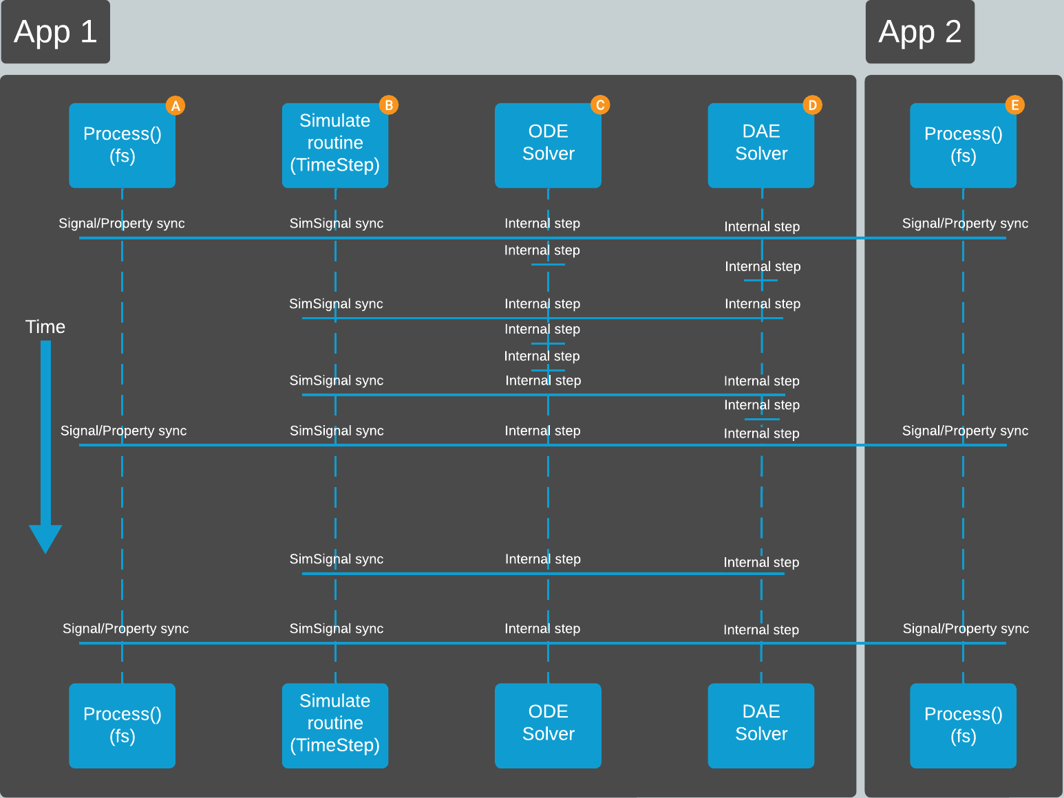
and During the SimulatorManager ProcessSimulate() call (frequency is determined by the SimulatorManager fs property), all values are synchronized and updated - both ordinary Signals and SimSignals, both simulator and normal control system components and even between different applications whether the applications are on the same physical computer or distributed over several computers in a local network. All integration methods are expected to provide new state variable values. Any CDPOperators not added under simulator components are processed and synced with the slower fs frequency set in their parent component.

During the Simulate routine (normally called multiple times by one ProcessSimulate()), routed SimSignals are synced between simulator components within the same application. Also, any CDPOperators added under the simulator components are processed and synced - this includes the FMI2Cosimulation operator in the case FMI models are used. All integration methods are expected to provide new state variable values.

The frequency of the Simulate routine is determined by the SimulatorManager TimeStep property. However, if the SimulatorManager AdaptiveTimeStep property is set to true, then the integration methods dynamically adjust the step size. In that case, TimeStep represents the minimum allowed time step, and the processing period (1 / fs) represents the maximum allowed time step. When the selected ODE and DAE integration methods request a different step size, the minimum of the two is used for the next step.

and The SimulatorManager is allowed to contain one ODE solver (integration method) for solving ordinary differential equations (ODEs) and one DAE solver (integration method) for solving differential-algebraic equations (DAEs). Both integration methods can take however many internal steps they need to meet the error tolerances configured in the integration method settings. A more detailed description is given in the Choosing an Integration Method manual.

Integration Methods

There are many algorithms for making a numeric solution to ordinary differential equations on the form

`dot y(t) = f(t, y(t)),`

`y(t_0) = y_0`

The main idea is to assume that the solution is linear within small enough time steps, i.e.

`y_{n+1} = y_n + a dt`

where `dt` is the time step, and `a` is the slope. The challenge is to find a good prediction of the slope.

Some systems also have algebraic constraints in addition to their differential components. In that case, they form differential-algebraic equations (DAEs) of the form `0 = g(t, y, dot y)`. CDPSim supports such systems by using a DAE solver that enforces these algebraic constraints at each step. They for example are useful when encountering algebraic loops.

CDPSim comes with several different integration algorithms and the user is able to add more algorithms by inheriting from IntegrationBase class. The available algorithms are listed on the Choosing an Integration Method page.

The integration method can be selected individually for each simulation application. The choice of algorithm and simulation time step depends on the nature of the simulated system. Stiff systems require smaller time steps, and to prevent instability, these (sub)systems should be implemented as separate applications to enable running them at smaller time steps, as running the complete system at a sufficiently small time step could be too CPU intensive for the host computer.

Foundation

Describing a Physical System

A physical system can be complex. To be able to simulate it, it is necessary to formulate a simplified model of the system, so simple that it is understandable for your mind and solvable for the computer, and so complex that it really can be used to tell something about the actual physical system you are investigating. Example 3: Long Elastic Wire is an example of how to make a model.

The behavior of the model is described in terms of differential equations. Deriving these requires some insight to physics, and is not always straight-forward. Two useful methods are presented.

Newtons Second Law

This is a well-known and widely used law. It states that the sum of all forces acting on a body is equal to the mass of the body times its acceleration, i.e. `sum F = ma`. `F` is a force, `m` is the mass, and `a` is the acceleration, which is the double time derivate of the position, `a = ddot x`. Then it is just a matter of finding the forces.

Consider for example a mass hanging from a spring, as one of the examples is simulating. The forces acting on the mass are the gravity force `G` and the spring force `S`. Gravity force is given by `G = mg`, where `m` is body mass and `g` is the gravity acceleration. Hooke's law states that the spring force is given by `S = -kx`, where `k` is a spring constant describing the stiffness of the spring, and `x` is the displacement from equilibrium (where the spring is at rest). The sum of forces is `sum F = G + S = mg - kx`. Newtons second law now yields that `mg - kx = m ddot x` which is a differential equation. Expressed in terms of `ddot x`, this yields

`ddot x = g - (k)/(m) x`

Euler-Lagrange Equations

In more complex systems, in particular rotating systems, it can be hard to identify all forces. Another way of deriving differential equations is to consider the energy of the system, and then apply the Euler-Lagrange equations. There are two main types of mechanical energy: kinetic energy `T` (energy from movement, for example a driving car) and potential energy `V` (for example energy associated with position in the gravitational field, like a bike on the top of a hill). The Lagrangian of a system is defined as the difference between these two energy types, i.e. `L = T - V`. The Euler-Lagrange equations is now

`(d)/(dt) ((del L) / (del dot q_i)) - (del L) / (del q_i) = 0`

where `q_i` are generalized coordinates, for example `x` in a one-dimensional movement. The challenge is thus to find the energy of the system.

Consider again the mass hanging from a spring. The kinetic energy of the mass is `T = 1/2 mv^2` . The potential energy due to displacement from spring equilibrium and gravitational energy is `V = 1/2 kx^2 - mgx`. Then the Lagrangian is

`L = T - V = 1/2 m dot x^2 - 1/2 k x^2 + mgx`

Now the Euler-Lagrange equation yields

`m ddot x + kx - mg = 0 rArr ddot x = g - k/m x`

just as we found by Newtons second law.

One might point out that in this example, Newtons second law seems to be by far the easiest way to derive the equations. In other cases, however, like the rotary inverted pendulum, it would be close to impossible to find the equations from Newtons second law. The Euler-Lagrange equations is thus a tangled, but more powerful method for deriving differential equations.

Developing First Order Differential Equations

The numerical integration methods available in CDPSim only deal with first order differential equations. Many physical systems, like the mass hanging from a spring, are however described by second order differential equations. Fortunately, all second order differential equations can easily be rewritten as two first order equations, simply by introducing a new state variable equal to the time derivative of the existing state variable.

Consider the second order differential equation describing the mass hanging from a spring:

`ddot x = g - k/m x`

Introduce a new variable `v` equal to the time derivative of `x`, and substitute the time derivatives of `x` in the equation with this new variable:

`dot x = v`

`dot v = g - k/m x`

We now have first order differential equations, ready to be implemented in CDPSim.

Developing Differential-Algebraic Equations

Most ODEs can be converted to algebraic equations subtracting the right-hand side of the differential equation from the left-hand side. E.g. the differential equation x.ddt = v; can be converted to the algebraic equation

x.residual = x.ddt - v;

This is often used when an ODE-based equation introduces an algebraic loop that typical ODE solvers cannot resolve.

Real-time Performance

One of the main advantages of CDPSim, is that the simulations can run in real time. However, if the simulation gets too CPU intensive, real-time simulation can not be achieved. This occurs if the integration time step is too small, or the code is too heavy to run, either because of a large number of components, or long loops in the code due to large state variable arrays. See Measuring Performance for information on measuring the performance of the simulation.

There are some options to deal with the performance problem:

• If using the no-code approach, recreate the simulation model in C++.
• Adjust the integration time step in the SimulatorManager component.
• Distribute the components to run on different computers.

Adjusting Integration Time Step in CDPSim

The integration time step can, just as the choice of integration algorithm, be adjusted in the SimulatorManager component by changing the TimeStep property.

Choosing a too small time step results in loss of real-time performance, while when using a too large time step, the solution of the differential equation becomes inaccurate, or the integration even blows up, and the program breaks down (for oscillating systems).

The limit where the integration becomes unstable is related to the highest underlying frequency in the system. Consider Example 3: Long Elastic Wire. Here, this highest frequency `f` is given by

`f = n sqrt{k / m}`

It is found that for the Runge-Kutta algorithm, the integration becomes unstable when

`dt approx sqrt{2}/f`

where `dt` is the integration time step.

Distribution of Components

A system consisting of many components can easily be distributed to run on different computers, simply by putting them to different CDP applications and routing the signals between them. Be aware that the routing frequency is limited to the process frequency of your SimulatorManager component. This is controlled by the fs property (which is different from simulation frequency controlled by TimeStep). The fs is usually around 100 Hz but may be increased to 10 kHz. On the other hand, if simulator components within the same application route SimSignals and StateVariables, then data is up to date regardless of process frequency.

A single component can also be split up for distributing purposes. For example, the mass-spring system (example 1) could be programmed such that one component handles the first half of the masses, and the second component handling the rest, routing the state variables through some additional signals. A major problem arises though, if the underlying frequency of the system is getting close to the process frequency, which might be the case for stiff systems. The process frequency can be increased if necessary, and it can also be an idea to find the slowest changing point in the system, and make the split here.

Further Reading

For further information, see the Getting Started, CDP Simulator Examples and Configuration Manual. For integration with other simulation tools using the Functional Mock-up Interface (FMI) standard, see FMI Co-Simulation Support.