Choosing an Integration Method
Introduction
CDPSim provides a variety of algorithms for solving ordinary differential equations (ODEs) and differential-algebraic equations (DAEs).
The user is able to add more algorithms by inheriting from CDPSim::IntegrationBase class.
ODE Algorithms
There are many algorithms for making a numeric solution to ordinary differential equations (ODE) on the form
`dot y(t) = f(t, y(t)),`
`y(t_0) = y_0`
The main idea is to assume that the solution is linear within small enough time steps, i.e.
`y_{n+1} = y_n + a dt`
where `dt` is the time step, and `a` is the slope. The challenge is to find a good prediction of the slope.
The following integration algorithms are available in CDPSim for solving ordinary differential equations (ODEs):
| Algorithm | Order | Concept | Internal State | Dense Output | Error Estimation / Controlled Stepper | CPU Usage | Usage Suggestions |
|---|---|---|---|---|---|---|---|
| Euler | 1 | Explicit | No | No | No | Very low | Useful for testing, very simple but not accurate for most purposes. |
| Heun | 2 | Explicit | No | No | No | Low | Improved Euler; a good step up from the simplest method. |
| RungeKutta4 | 4 | Explicit | No | No | No | Moderate | The default in CDPSim; a good trade-off between speed and accuracy. |
| Bulirsch-Stoer (Boost.Odeint) | Variable (1-16) | Explicit | No | Yes | Yes (Adaptive) | High | Very good if high precision is required. |
| Cash-Karp (Boost.Odeint) | 5 | Explicit | No | No | Yes (4) | Moderate | Non-stiff systems; good balance of accuracy and performance. |
| Dormand-Prince (Boost.Odeint) | 5 | Explicit | Yes | Yes | Yes (4) | Moderate | Non-stiff systems; widely used due to effective error control and moderate overhead. |
| Fehlberg (Boost.Odeint) | 8 | Explicit | No | No | Yes (7) | Very high | Non-stiff, smooth models; more computational effort per step but can reduce total steps needed for high-accuracy solutions; ideal when very high accuracy is essential. |
| Rosenbrock4 (Boost.Odeint) | 4 | Implicit | No | Yes | Yes (Adaptive) | Very high | Good for stiff problems; more expensive per step due to Jacobian evaluations but stable for stiff problems. |
| CVODE Adams (SUNDIALS) | Variable (1-12) | Implicit | Yes | Yes | Yes (Adaptive) | Moderate | Non-stiff ODEs; variable order and adaptive steps for efficient integration. |
| CVODE BDF (SUNDIALS) | Variable (1-5) | Implicit | Yes | Yes | Yes (Adaptive) | Moderate | Stiff ODEs; robustness and adaptive order make it suitable for difficult problems. |
Definitions:
- Order: The order of the method, indicating the error per time step.
- Concept: Whether the method is explicit (computes the next step purely from known values) or implicit (may require solving equations involving unknown future states, often used for stiff problems).
- Internal State: Whether the method keeps an internal state of old derivatives for better error control.
- Dense Output: Whether the method can provide output at intermediate points between its internal steps to match exactly the SimulatorManager TimeStep.
- Error Estimation / Controlled Stepper: Whether the method has an embedded method for error estimation and the order of the estimate (in parentheses). If present, a controlled stepper will be used, which utilizes the error estimates to adjust the step size automatically, ensuring the integration meets accuracy requirements with minimal user intervention.
- CPU Usage: Indicates the relative CPU usage compared to other methods.
- Stiff System: A system of ODEs whose solutions involve very rapid changes alongside slower dynamics, forcing explicit methods to take extremely small time steps for stability. Stiff problems typically benefit from implicit solvers.
Note: The CPU usage comparison assumes the same SimulatorManager TimeStep is used for all algorithms. However, higher-order methods can often use larger time steps, potentially resulting in lower overall CPU usage while achieving the same accuracy as simpler methods. See Measuring Performance for information on how to monitor the simulator's CPU usage.
DAE Algorithms
Differential-algebraic equations (DAEs) solve equations in the form
`0 = f(y,dot y,t)`
Note: DAE solver is only used for components where the property SolverType is set to Algebraic (DAE).
Behavior:
- DAE is intended for algebraic constraints that cannot be handled by standard ODE solvers, such as equations containing algebraic loops.
- It computes residuals (the difference between the current algebraic constraint and its desired value) rather than derivatives.
- The solver will iterate to ensure these residuals converge to zero, effectively solving any algebraic loops.
The following is available in CDPSim for solving differential-algebraic equations (DAEs):
| Algorithm | Order | Concept | Internal State | Dense Output | Error Estimation / Controlled Stepper | CPU Usage | Usage Suggestions |
|---|---|---|---|---|---|---|---|
| SUNDIALS IDA | Variable (1-5) | Implicit | Yes | Yes | Yes (Adaptive) | Moderate | Problems where ODE solvers fail due to algebraic loops or other constraints. |
Initial Conditions
For ODE solvers, the initial conditions are given by the initial values of the state variables (set in Configure mode by the Value property in a CDPSim::StateVariable) or by the State node in the Integrator block. For DAE solvers however, it is also recommended to set initial values to the ddt property of the state variables to ensure the solver has a good starting point.
DAE Applications
Here are some typical applications where DAEs are used:
| Application | Differential Components | Algebraic Constraints | Real-Time Control Need | Why DAE Instead of ODE? |
|---|---|---|---|---|
| Power Systems (Synchronous Generators) | Generator swing dynamics | Power flow constraints (Kirchhoff's laws) | Grid stability under fluctuating loads | Kirchhoff's laws enforce instantaneous constraints on voltage and current, requiring DAEs instead of pure ODEs. |
| Robotics (Parallel & Industrial Robots) | Joint motion dynamics | Kinematic constraints | Precise motion planning with constraints | The kinematic constraints define fixed relationships between joint positions, preventing reduction to ODEs. |
| Vehicle Suspension (Active Suspension Systems) | Chassis and wheel dynamics | Road contact constraints | Comfort & stability in variable terrain | Road contact constraints must be continuously enforced to prevent penetration or separation, requiring algebraic conditions in a DAE. |
| Marine Systems (Dynamic Positioning) | Ship motion in 6-DOF | Hydrodynamic and thruster constraints | Precise station-keeping against disturbances | Thruster force allocation involves algebraic equations that must be solved along with dynamic equations. |
| Aircraft Systems (Fly-by-Wire Flight Control) | Rigid-body flight dynamics | Aerodynamic force constraints | Stability control under dynamic conditions | Aerodynamic force and moment constraints impose equilibrium conditions that cannot be represented solely by ODEs. |
| Hydraulic Accumulator (Van der Waals Gas Model) | Gas volume dynamics | Van der Waals equation constraints | Pressure regulation for fluid power storage | The gas pressure must satisfy the nonlinear Van der Waals equation at all times, making the system a DAE rather than an ODE. |
| Rotary Inverted Pendulum | Angular motion dynamics | Torque and linkage constraints | Balance control and stabilization | The constraints on the rotating arm and pendulum introduce coupled algebraic equations that must be solved along with the differential equations of motion. |
Setting the Integration Algorithm
In a simulation application, the integration algorithm is set in the SimulatorManager component by adding a new row into the Integration table from the Resource tree.
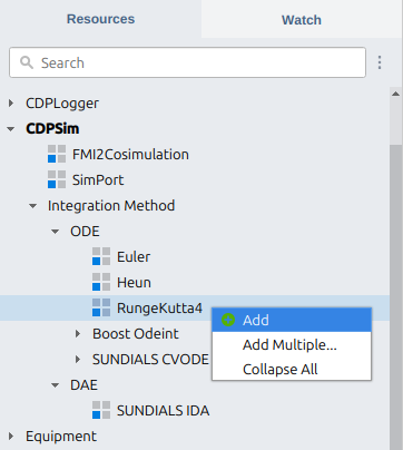
Only one ODE and only one DAE integration algorithm can be added to each application. When an integrator is not specified, the SimulatorManager will default to RungeKutta4 for ODE and SUNDIALS IDA for DAE.
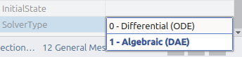
By default, the simulator components use the ODE integration algorithm. To use the DAE solver, each simulator component has a SolverType property which can be set to Algebraic (DAE).
The choice of algorithm and simulation time step depends on the nature of the simulated system. Stiff systems require smaller time steps, and to prevent instability, these (sub)systems should be implemented as separate applications to enable running them at smaller time steps, as running the complete system at a sufficiently small time step could be too CPU intensive for the host computer.
Note: When separating components into different applications, the values between applications will be synchronized at the frequency set by SimulatorManager fs property. However, simulator values within the application will be synchronized at a much higher rate (set by SimulatorManager TimeStep property). This means it is only worth separating components which are not tightly coupled.
For more information on creating a simulation application and configuring it, see the Getting Started and Configuration Manual pages.
Detailed Description
Euler Method
The Euler method simply states that the next `y`-value approximately equals the previous value plus the time derivative of `y` times a chosen time step `dt`:
`y_{n+1} = y_n + f(t_n,y_n) dt`
This method introduces an error per time step proportional to `dt^2`, which results in a total error in the order of magnitude `dt` when solving over a given range of `t`. The Euler method is thus said to be a first-order method.
Heun's Method (Improved Euler's Method)
Heun's method is a so-called predictor-corrector method, using Euler's method as a predictor and a trapezoidal method as a corrector. The idea is to first calculate an intermediate value, and then weigh this value equally with the previous value when calculating the value at the next time step:
`tilde y_{n+1} = y_n + f(t_n,y_n) dt` (intermediate value)
`y_{n+1} = y_n + 1/2 ( f(t_n,y_n) + f(t_{n+1}, tilde y_{n+1}) ) dt`
The error is here proportional to `dt^3`.
Runge-Kutta Method
The Runge-Kutta method has a more comprehensive way of predicting the slope, given by the following equation:
`y_{n+1} = y_n + 1/6 ( k_1 + 2 k_2 + 2 k_3 + k_4 ) dt`
where
`k_1 = f (t_n, y_n)`
`k_2 = f (t_n + 1/2 dt, y_n + 1/2 k_1 dt)`
`k_3 = f (t_n + 1/2 dt, y_n + 1/2 k_2 dt)`
`k_4 = f (t_n + dt, y_n + k_3 dt)`
This method produces an error of order `dt^5`.
Boost Odeint
The Boost odeint library is a collection of algorithms for solving ordinary differential equations.
BulirschStoer
The Bulirsch-Stoer is a variable-order (1-16) method. It is one of the most complex and powerful methods provided by odeint. A highly adaptive method to be used if high precision is required. Supports dense output and uses error estimation for controlled stepping.
CashKarp
The CashKarp method is a good general scheme with error estimation for nonstiff problems. It is a fifth-order Runge-Kutta method with an embedded fourth-order method for error estimation.
DormandPrince
The Dormand-Prince is a standard method with error control and dense output for nonstiff problems. It is a fifth-order Runge-Kutta method with an embedded fourth-order method for error estimation. It is very similar to the Cash-Karp method (same order and same number of evaluations per step), but has dense output capability meaning it can provide output at intermediate points between its internal steps to match exactly the SimulatorManager TimeStep.
Commonly used in solving ordinary differential equations due to its balance between accuracy and computational cost.
Fehlberg
The Fehlberg is a good high-order method with error estimation for smooth, nonstiff problems. It is an eight-order Runge-Kutta method with an embedded seventh-order method for error estimation. It is ideal when very high accuracy is essential.
RosenBrock4
The Rosenbrock4 method is an implicit fourth-order method with dense output and error estimation for controlled stepping. It is particularly well-suited for stiff problems where stability is a concern.
Properties
The following properties can be set for the Boost odeint solvers:
| Property | Description |
|---|---|
| RelativeTolerance | The scalar relative tolerance, see the Tolerances paragraph for more information. |
| AbsoluteTolerance | The absolute tolerance for the solver, see the Tolerances paragraph for more information. |
| MaxTimeStep | Maximum allowable internal step size for the solver, set to 0.0 to default to SimulatorManager's max. See the Adaptive Time Step paragraph for more information. |
| InternalStepsPerCycle | Number of steps taken by the solver within one SimulatorManager process cycle (determined by the SimulatorManager's fs property). For steppers with error estimation, this shows if they reduced the internal step size to meet specified RelativeTolerance and AbsoluteTolerance. Note, the maximum step size is determined by SimulatorManager's TimeStep property (not fs). |
SUNDIALS CVODE
The SUNDIALS suite is a collection of numerical algorithms for solving ordinary differential equations. The CVODE solver is a part of the SUNDIALS suite and is used in CDPSim to solve ordinary differential equations.
The CVODE solver supports two different methods for solving ordinary differential equations: Adams-Moulton and BDF.
- Adams-Moulton - A multistep method for solving ordinary differential equations. Particularly suited for non-stiff problems.
- Backward Differentiation Formula (BDF) - A multistep method for solving stiff ordinary differential equations.
The error produced by the CVODE solver is controlled by the relative and absolute tolerances, which can be set by the user by setting the properties RelativeTolerance and AbsoluteTolerance.
It is also possible to set the minimum and maximum step sizes for the CVODE solver using the properties MinTimeStep and MaxTimeStep. When set to 0, for MinTimeStep, the CVODE default is used which has been tuned for a wide range of problems and has a long history of success. The default value for MaxTimeStep is set to SimulatorManager's default to prevent the solver from interfering with the CDP Framework's signal synchronization.
The maximum order of the integration method can be set using the property MaxOrder. When set to 0, it defaults to 12 for Adams and 5 for BDF formulas, which are the maximum values allowed for MaxOrder.
Stability Limit Detection (BDF only)
At order 1 or 2, the BDF method is A-stable. This means that, roughly speaking, as long as all modes in the system are stable, the method is also stable for any choice of step size, at least in the sense of a local linear stability analysis. At orders 3 to 5, the BDF methods are not A-stable, although they are stiffly stable. The size of the region of instability grows as the order increases from 3 to 5.
The stability limit detection algorithm works directly with history data that is readily available in CVODE. If it concludes that the step size is in fact stability-limited, it dictates a reduction in the method order, regardless of the outcome of the error-based algorithm. This option adds some computational overhead (about 2% to 7%). But if the step sizes are being limited by stability then turning on the option will improve the efficiency of the solution.
Read more at CVODE documentation.
Properties
The following properties can be set for the CVODE solver:
| Property | Description |
|---|---|
| RelativeTolerance | The scalar relative tolerance, see the Tolerances paragraph for more information. |
| AbsoluteTolerance | The absolute tolerance for the solver, see the Tolerances paragraph for more information. |
| MinTimeStep | Minimum allowable step size for the CVODE solver, set to 0.0 to use the CVODE default. See the Adaptive Time Step paragraph for more information. |
| MaxTimeStep | Maximum allowable step size for the CVODE solver, set to 0.0 to default to SimulatorManager's max. See the Adaptive Time Step paragraph for more information. |
| MaxOrder | Maximum order of the integration method. When set to 0, it defaults to 12 for Adams and 5 for BDF formulas. An input value greater than the default will result in the default value. |
| MaxNumSteps | The maximum number of internal steps that CVODE can take between two output points. This prevents the solver from stalling in extremely small time steps or entering an infinite loop. Increase this when encountering CV_TOO_MUCH_WORK error. |
| InternalStepsPerCycle | Number of steps taken by the solver within one SimulatorManager process cycle (determined by the SimulatorManager's fs property). For steppers with error estimation, this shows if they reduced the internal step size to meet specified RelativeTolerance and AbsoluteTolerance. Note, the variable step size is limited by MinTimeStep and MaxTimeStep properties. |
| StabilityLimitDetection (BDF only) | Enable (true) or disable (false) stability limit detection in the CVODE solver for BDF formula. Useful for stiff problems to enhance performance. |
SUNDIALS IDA
The SUNDIALS suite also provides the IDA solver, which is used in CDPSim for solving differential-algebraic equations (DAEs). In contrast to the CVODE solver that handles ordinary differential equations, IDA is specifically designed to manage systems of the form
`F(t, y(t), dot y(t)) = 0`
`y(t_0) = y_0`
`dot y(t_0) = dot y_0`
IDA uses variable-step, variable-order (1-5) implicit methods based on the backward differentiation formulas (BDF). Because these formulas are implicit, IDA is especially well-suited for stiff or moderately stiff DAEs. Like CVODE, IDA incorporates an internal error control mechanism guided by user-defined tolerance settings, ensuring that each time step is taken as large as possible while still meeting the specified accuracy.
The algebraic nature of some of the equations requires satisfying constraints at each step, so the solver must ensure that both differential and algebraic components remain consistent. IDA manages this through its internal initialization routines, which can adjust initial conditions to achieve consistency if required.
Properties
The following properties can be set for the IDA solver:
| Property | Description |
|---|---|
| RelativeTolerance | The scalar relative tolerance, see the Tolerances paragraph for more information. |
| AbsoluteTolerance | The absolute tolerance for the solver, see the Tolerances paragraph for more information. |
| MinTimeStep | The minimum allowable step size for the IDA solver, set to 0.0 to let IDA use its own default. See the Adaptive Time Step paragraph for more information. |
| MaxTimeStep | The maximum allowable step size for the IDA solver, set to 0.0 to default to SimulatorManager's max. See the Adaptive Time Step paragraph for more information. |
| MaxOrder | The maximum order of the integration method. For the BDF formulas in IDA, the typical maximum order is 5. An input value greater than 5 will still default to 5. |
| MaxNumSteps | The maximum number of internal steps that IDA can take between two output points. This prevents the solver from stalling in extremely small time steps or entering an infinite loop. Increase this when encountering IDA_TOO_MUCH_WORK error. |
| InternalStepsPerCycle | Number of steps taken by the solver within one SimulatorManager process cycle (determined by the SimulatorManager's fs property). For steppers with error estimation, this shows if they reduced the internal step size to meet specified RelativeTolerance and AbsoluteTolerance. Note, the variable step size is limited by MinTimeStep and MaxTimeStep properties. |
Just as with CVODE, fine-tuning these properties (including tolerances and step-size settings) is often necessary for optimizing simulation speed and ensuring that the solver's accuracy requirements are met for a given system of DAEs.
General Recommendations
Tolerances
The relative and absolute tolerances are crucial for the performance of the integration. The tolerances should be set according to the problem at hand. If the tolerances are too tight, the integration method will take more steps to reach the same solution, which will increase the CPU usage. If the tolerances are too loose, the method will take fewer steps, but the solution will be less accurate.
See also: the SUNDIALS FAQ about choosing tolerances.
Relative Tolerance
The relative tolerance is a scalar value that controls the relative errors. A value of 1e-4 means that errors are controlled to 0.01%. It is not recommended to use a relative tolerance larger than 1e-3. On the other hand, the relative tolerance should not be so small that it is comparable to the unit roundoff of the machine arithmetic (generally around 1e-15).
The final (global) errors are an accumulation of per-step errors. A good rule of thumb is to reduce the tolerances by a factor of 100 from the actual desired limits on errors. So if you want 0.01% accuracy (globally), a good choice is 1e-6 for the relative tolerance.
Absolute Tolerance
The absolute tolerance is used to control absolute errors when any components of the solution vector y may be so small that pure relative error control is meaningless. For example, if y[i] starts at some nonzero value but decays to zero, then pure relative error control on y[i] makes no sense (and is overly costly) after y[i] is below some noise level. It is impossible to give any general advice on absolute tolerance values because the appropriate noise levels are completely problem-dependent.
Adaptive Time Step
Some integration methods support adaptive time steps. The adaptive time step is a powerful feature that allows the method to adjust the time step size based on the error estimate and the user-defined relative and absolute tolerances. This can be useful when the system has varying dynamics, as the integration method can take larger steps when the system is stable and smaller steps when the system is unstable. This can reduce the CPU usage while maintaining similar accuracy.
Note: Only integration methods with error estimation and controlled stepper support adaptive time steps, see the table in the Introduction. In addition, many of them only support configuring the maximum internal time step the solver can take while the minimum internal step size is determined by the configured error tolerances.
If the SimulatorManager AdaptiveTimeStep property is enabled, the integration method will adjust not just its internal step size but also the time step of the Simulate routine, affecting the synchronization frequency of SimSignals routed between simulator components. For more details on the AdaptiveTimeStep property, refer to the Configuration Manual.
Minimum Time Step
The minimum time step is the smallest time step the integration method is allowed to take. It is useful to limit this value to make sure the simulation does not fall behind real time.
Note, while the method can take smaller steps internally, the SimulatorManager TimeStep property sets the minimum step size for the Simulate routine.
Maximum Time Step
The maximum time step is the largest time step the integration method is allowed to take. It is useful to limit this value to prevent the method from taking too large steps, which can lead to instability.
When the SimulatorManager AdaptiveTimeStep property is disabled, the maximum time step is determined by the SimulatorManager TimeStep property. This is the time step at which routed SimSignals are synchronized between the simulator components as part of the Simulate routine.
On the other hand, when the SimulatorManager AdaptiveTimeStep property is enabled, the integration method can adjust the time step of the SimulatorManager to control SimSignal synchronization frequency between simulator components. However, there is still a limit to how large the time step can be set, which is determined by the SimulatorManager fs property (the processing frequency), meaning the maximum step size is 1 / fs. This is the frequency at which other CDP components expect to receive data from the simulator and it is not practical for the integration method's step to exceed this period.
When inheriting from CDPSim::IntegrationBase, the SimulatorManager maximum time step can be queried with the SimulatorManager::GetSimulatorMaxTimestep() method.
Algebraic Loops
When using implicit ODE solvers like SUNDIALS CVODE or Boost RosenBrock4, it is important to note that the solvers are not able to handle algebraic loops. An algebraic loop in a simulation occurs when outputs depend directly on themselves without any delay, creating an implicit equation that must be solved at each time step.
For instance, the Example 2: Rotary Inverted Pendulum could be implemented with a simpler formula where dtheta.ddt and dphi.ddt are coupled. Each equation contains both dtheta.ddt and dphi.ddt. This means that to compute dtheta.ddt, we need to know dphi.ddt, and vice versa. The code below illustrates this:
void YourModelName::EvaluateDiffEquations(double t)
{
    theta.ddt = dtheta;
    phi.ddt = dphi;
    dtheta.ddt = 6.0 / (7.0 * l)
        * (g * sin(theta) - r * dphi.ddt * cos(theta) - 2.0 / (m_rod * 1) * c_rod * dtheta);
    dphi.ddt = 1.0 / (r * r * (m_rod + (1.0 / 3.0) * m_arm))
        * (0.5 * m_rod * r * l * dtheta * dtheta * sin(theta)
            - 0.5 * m_rod * r * l * dtheta.ddt * cos(theta) - c_arm * dphi + tau);
}
This interdependency forms an algebraic loop, transforming the system into a set of Differential-Algebraic Equations (DAEs) rather than pure Ordinary Differential Equations (ODEs). The loops introduce implicit dependencies that require solving nonlinear systems at each time step. In this case, some implicit solvers like the CVODE will fail with a CV_CONV_FAILURE error while others like the Boost RosenBrock4 will attempt to solve but can use 10 times more CPU time compared to a system without algebraic loops and often trigger the NotRealTime alarm.
Time Delay
One way to resolve algebraic loops is to introduce a time delay. This can be done by storing the previous value of the dependent variable and using it in the calculation. This will break the algebraic loop and allow the solver to proceed. This however can introduce a delay in the system, which may or may not be acceptable.
Explicit ODE Solvers
If it is not possible to reformulate the equations to avoid the algebraic loop, one can try to use explicit solvers like Heun, RungeKutta4, or some of the other Boost odeint solvers. Explicit solvers can bypass or approximate the interdependence by evaluating the equations sequentially, albeit with potential stability issues if the time step is too large. These methods essentially guess the solution at each step without fully resolving the algebraic loop. In systems with tight coupling, this can work reasonably well if the time step is small enough.
DAE Solvers
A better solution however would be to set your component to use a DAE solver. In Configure mode, set the property SolverType to Algebraic (DAE) and in Code mode implement the EvaluateAlgebraicEquations method to calculate the residuals of the algebraic equations:
void YourModelName::EvaluateAlgebraicEquations(double t)
{
    theta.residual = theta.ddt - dtheta;
    phi.residual = phi.ddt - dphi;
    dtheta.residual = dtheta.ddt - (6.0 / (7.0 * l)
        * (g * sin(theta) - r * dphi.ddt * cos(theta) - (2.0 * c_rod / m_rod) * dtheta));
    dphi.residual = dphi.ddt - (1.0 / (r * r * (m_rod + (1.0 / 3.0) * m_arm))
        * (0.5 * m_rod * r * l * dtheta * dtheta * sin(theta)
            - 0.5 * m_rod * r * l * dtheta.ddt * cos(theta) - c_arm * dphi + tau));
}
Tip! Most ODEs can be converted to algebraic equations by subtracting the right-hand side of the differential equation from the left-hand side. E.g. the differential equation x.ddt = v; can be converted to the algebraic equation x.residual = x.ddt - v;.
Get started with CDP Studio today
Let us help you take your great ideas and turn them into the products your customer will love.