Simulating Spring–Mass System
Introduction
The purpose of this example is to demonstrate a basic CDP Simulator project in CDP Studio, the independent automation software for open PC-based real-time distributed control systems. The purpose is also to show how to implement the simulator in different ways through code, low-code and no-code and how performance is influenced by the different implementations.
The project shows how easy it is to create a custom mathematical model for simulation using a mass hanging from a spring as an example.
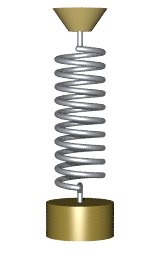
Mass-spring Harmonic Oscillator (Svjo / © CC BY-SA 3.0)
Project Overview
This example includes:
- A library project containing one simulator component - a C++ class that implements the mathematical model of a mass hanging from a spring.
- A system project containing 3 simulator applications that provide 3 different implementations for the mass-spring model:
- The SpringSimulatorCpp application uses the C++ simulator component created in the library project.
- The SpringSimulatorNoCode application uses no-code blocks like CDPOperators and Integrators to achieve the same result.
- The SpringSimulatorLowCode application uses the Evaluate operator to calculate the acceleration of the mass based on the spring force and damping. The integration part is still done using the no-code Integrator blocks.
Note: For each simulator application, the SimulatorManager Activate property has been set to 2 to slightly delay the simulation start. This ensures that for the no-code and low-code solutions, the initial values have propagated through the routing system between the no-code blocks.
How the Example Was Made
There is a more detailed explanation of the example available in the CDPSim manual, see Example 1: Mass Hanging from a Spring.
Implementations
Consider a mass hanging from a spring. The mathematical model is:
`dot x = v`
`dot v = - x k/m - v b/m`
The position `x` denotes the displacement from spring equilibrium and `v` is the speed of the mass hanging from the spring. Parameter `m` specifies the mass of the body, `k` is the spring constant and `b` the damping coefficient.
Code-based Implementation
A differential equation like this can be evaluated when inheriting from the DynamicSimComponent class and implementing the EvaluateDiffEquations method.
void MassSpring::EvaluateDiffEquations(double t)
{
    x.ddt = v;
    v.ddt = -x * k/m - v * b/m;
}
The full implementation of the code-based model is available in the MassSpring.cpp file. To open it, navigate to the Code mode and expand the SimulationLib project.
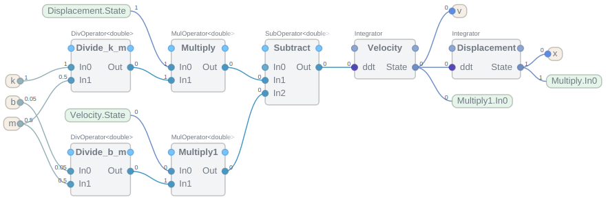
No-Code Implementation
The no-code solution uses a series of CDPOperator blocks to calculate the acceleration of the mass. The acceleration is then integrated using the Integrator blocks.
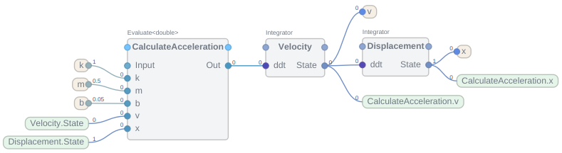
Low-Code Implementation
The low-code solution uses the Evaluate operator to calculate the acceleration of the mass using a simple script set to the Expression property of the operator.
-x * k/m - v * b/m
The acceleration is then integrated using the Integrator blocks.
Moving the mathematical formula of calculating the acceleration to a script helps avoid cluttering the view with too many multiplication and division operator blocks while still keeping the flexibility and simplicity of the no-code solution.
Note: The low-code solution often has better performance than the no-code solution because it reduces the number of value routings.
How to Run the Example
To run the example from CDP Studio, open Welcome mode and find it under Examples. Next, in Configure mode right-click on the library project and select Build, then right-click on the system project and select Run & Connect. See the Running the Example Project tutorial for more information.
The Graph application will now visualize the damped oscillation of the mass as provided by the 3 implementations.
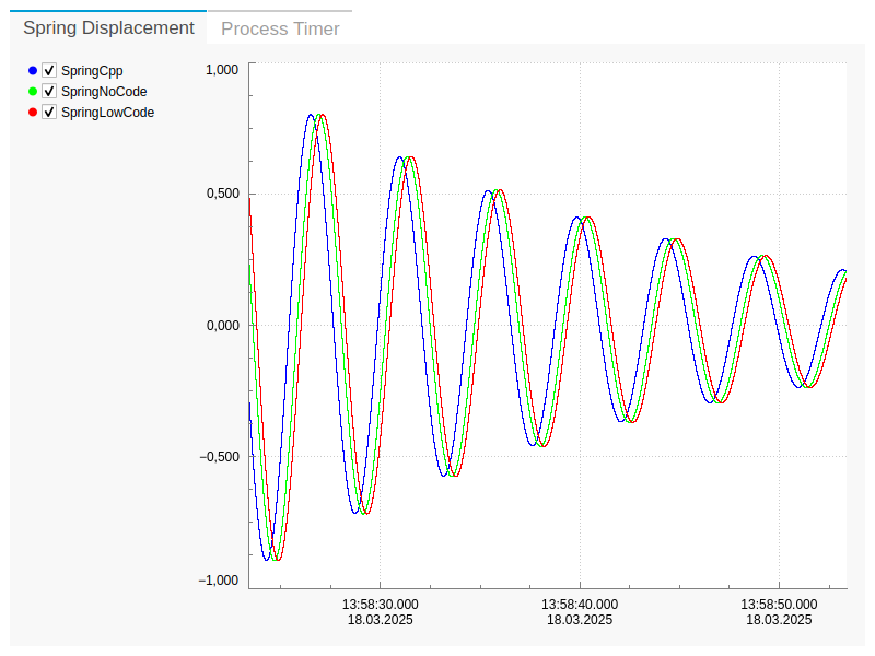
Note: The three graphs are off-sync because they are all separate application binaries and the startup time is a bit random. To synchronize them, one could disable the Autostart property of the SimulatorManager component in each application and programmatically send the Start message to each SimulatorManager at the same time but this is out of the scope of this example.
Measuring Performance
Having three distinct implementations of the same mathematical model allows us to compare the performance of each solution. As described in the Measuring Performance section of the CDPSim manual, plotting the Process Timer signal of the SimulatorManager component will show the simulator load on a scale from 0 to 1.
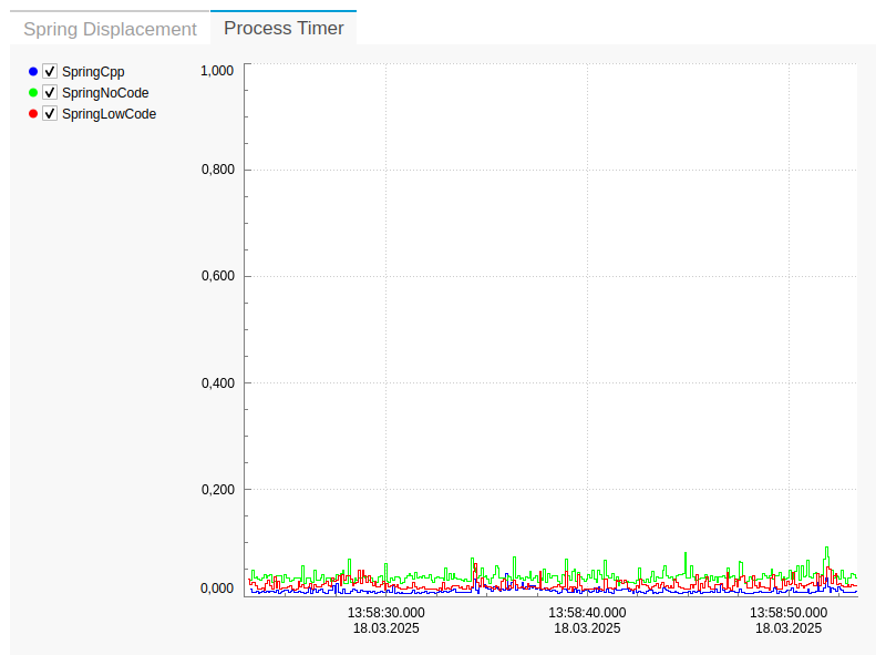
Usually, the C++ implementation will be the fastest, followed by the low-code solution. The no-code solution will be the slowest due to the overhead of the many extra routings between the operator blocks. When the simulator falls behind real-time, consider lowering the SimulatorManager sampling frequency (fs) and increasing the step size (TimeStep).
Integration Methods
When no integration method is specified, the SimulatorManager component defaults to using the Runge-Kutta Method with the default options.
To customize the integration method or to edit the default options, one must manually add an Integration Method from the Resource tree to the SimulatorManager component. See the Setting the Integration Algorithm section of the CDPSim manual for more information.
Read More
For further information see the CDP Simulator manual.
Get started with CDP Studio today
Let us help you take your great ideas and turn them into the products your customer will love.